Analyzing 10 Years of Eurojackpot Data with Python's Polars (Spoiler: It Doesn't Help)

Welcome to the intersection of high-performance data engineering and terrible financial decisions.

In this post, we are going to do what every hopeful gambler eventually tries: analyze historical lottery data to find the “secret pattern.” To do this, we will use Python’s Polars library—because if we are going to calculate our inevitable financial ruin, we might as well do it with blazing fast, multi-threaded performance.

Spoiler alert: the data won’t help you win. But it is a fantastic exercise in data manipulation, nested JSON parsing, and visualization. Let’s dive in.

Step 1: Setup Your Development Environment

To follow along, you will need a Python environment with Polars (for data crunching) and Matplotlib (to draw pretty charts of our losses). Run this in your terminal:

mkdir eurojackpot-analysis
cd eurojackpot-analysis
python -m venv .venv
source .venv/bin/activate
pip install polars matplotlib

Step 2: Loading the Eurojackpot Draw History

We provide a massive, free dataset of all Eurojackpot draws over the last 10+ years right here on the site. Let’s grab it:

wget https://www.howtolosemoneyfast.com/downloads/eurojackpot-history.json

Step 3: The “Reality Check” Script

Here is the complete Python script. It uses Polars’ powerful .explode() method to untangle the nested arrays of winning numbers, and .unnest() to flatten the prize distribution data.

import polars as pl
import matplotlib.pyplot as plt
from pathlib import Path
from typing import Union

def load_lottery_data(file_path: Union[str, Path]) -> pl.DataFrame:
    """Loads historical lottery data from a JSON file."""
    path = Path(file_path)
    if not path.exists():
        raise FileNotFoundError(f"Dataset not found at: {path}")
    return pl.read_json(path)

def calculate_number_frequencies(df: pl.DataFrame, column_name: str, top_n: int = 10) -> pl.DataFrame:
    """Calculates the frequency of drawn numbers."""
    return (
        df.select(pl.col(column_name).explode())
        .group_by(column_name)
        .agg(pl.len().alias("frequency"))
        .sort("frequency", descending=True)
        .head(top_n)
    )

def analyze_payout_distribution(df: pl.DataFrame) -> pl.DataFrame:
    """Calculates summary statistics for minor prize tiers."""
    payouts_df = df.select(
        pl.col("date"), 
        pl.col("prizeDistribution")
    ).unnest("prizeDistribution")
    
    summary_stats = payouts_df.select([
        pl.col("2 + 1").drop_nulls().mean().round(2).alias("2 Main + 1 Euro"),
        pl.col("3 + 0").drop_nulls().mean().round(2).alias("3 Main + 0 Euro"),
        pl.col("3 + 1").drop_nulls().mean().round(2).alias("3 Main + 1 Euro")
    ])
    return summary_stats

def plot_reality_check(top_main: pl.DataFrame, payout_stats: pl.DataFrame):
    """Generates a professional dual-plot visualization."""
    
    # Set up a professional plotting style
    plt.style.use('ggplot')
    fig, (ax1, ax2) = plt.subplots(1, 2, figsize=(14, 6))
    fig.suptitle("Eurojackpot Historical Analysis: The Illusion of Strategy", fontsize=16, fontweight='bold')

    # --- Plot 1: "Hot" Numbers ---
    # Convert Polars columns to lists for Matplotlib
    numbers = [str(n) for n in top_main["mainNumbers"].to_list()]
    frequencies = top_main["frequency"].to_list()
    
    ax1.bar(numbers, frequencies, color='#2c3e50', edgecolor='black')
    ax1.set_title("Top 10 Most Frequent Main Numbers", fontsize=12)
    ax1.set_xlabel("Lottery Number")
    ax1.set_ylabel("Times Drawn")
    
    # Add a cynical watermark/text box
    ax1.text(0.05, 0.95, "Past performance does not\nindicate future results.", 
             transform=ax1.transAxes, fontsize=10, verticalalignment='top', 
             bbox=dict(boxstyle='round', facecolor='white', alpha=0.8))

    # --- Plot 2: Payout Reality ---
    # Extract column names and their single row values
    tiers = payout_stats.columns
    avg_payouts = payout_stats.row(0)
    
    ax2.bar(tiers, avg_payouts, color='#e74c3c', edgecolor='black')
    ax2.set_title("Average Payouts for Common 'Wins'", fontsize=12)
    ax2.set_xlabel("Matching Tiers")
    ax2.set_ylabel("Average Payout (€)")
    
    # Add exact values on top of the bars
    for i, v in enumerate(avg_payouts):
        ax2.text(i, v + 0.5, f"€{v:.2f}", ha='center', fontweight='bold')

    plt.tight_layout()
    
    # Save the plot so you can upload it straight to your blog
    output_filename = "eurojackpot_reality_check.png"
    plt.savefig(output_filename, dpi=300)
    print(f"\n[+] Chart successfully generated and saved as '{output_filename}'")
    
    # Show the plot window
    plt.show()

def main():
    pl.Config.set_tbl_formatting("ASCII_MARKDOWN")
    pl.Config.set_tbl_hide_column_data_types(True)
    
    file_path = "eurojackpot-history.json"
    
    try:
        print("Initializing Eurojackpot Historical Analysis...\n")
        df = load_lottery_data(file_path)
        
        # Get top 10 for a better looking chart
        top_main = calculate_number_frequencies(df, "mainNumbers", top_n=10)
        payout_stats = analyze_payout_distribution(df)
        
        # Generate the visualization
        plot_reality_check(top_main, payout_stats)
        
    except Exception as e:
        print(f"Analysis failed: {e}")

if __name__ == "__main__":
    main()

The Results

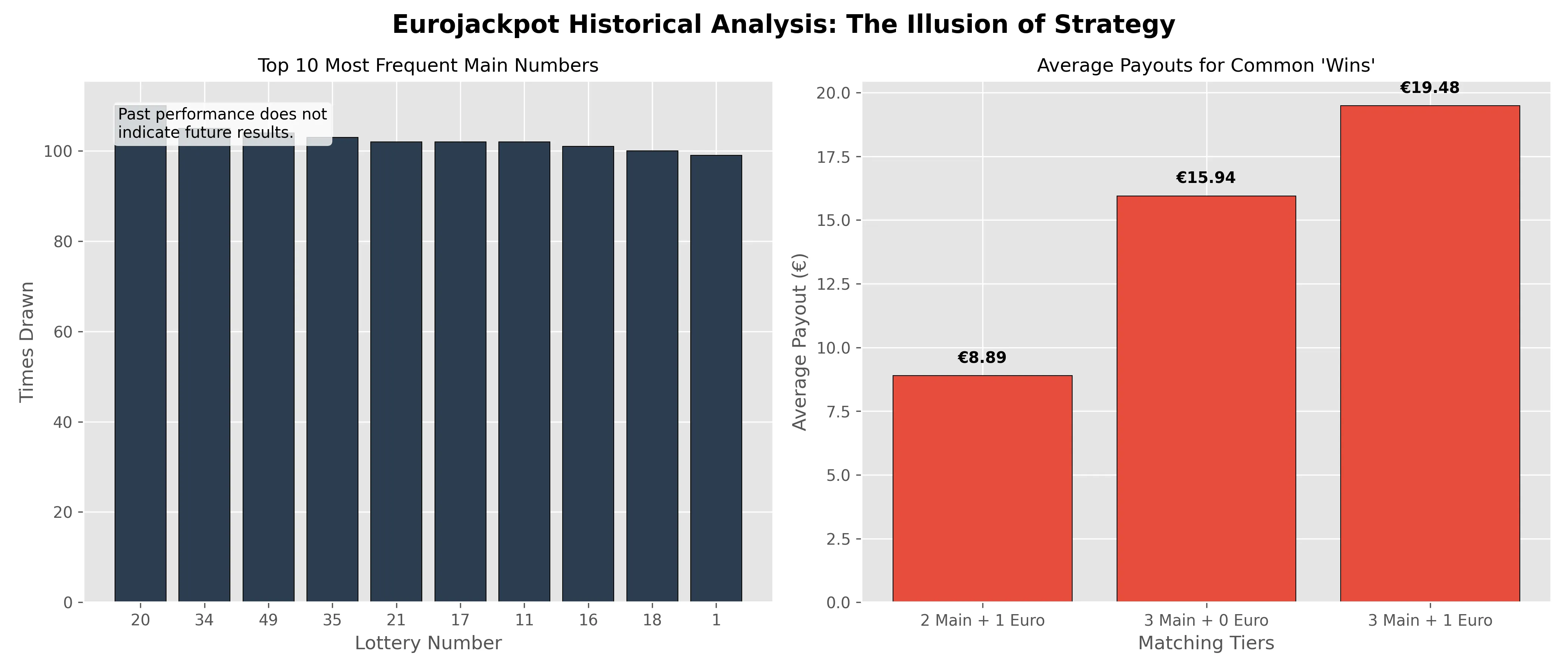
When you run this script, Matplotlib generates the following reality check:

The takeaway: Even if you successfully pick the “hottest” historical numbers, and you manage to match 3 Main numbers and 1 Euro number… congratulations. You’ve statistically won enough to buy a nice pizza.

Want to see the math in action without writing any code? Try running 1,000 lifetimes of tickets through our live Eurojackpot Simulator and watch your virtual bank account drain in real-time.