Monte Carlo Simulation: How to go broke eight times faster with 8 Eurojackpot lines

Every lottery player knows the saying: “One line is no line, you have to play a few more to boost your chances!” That’s why the average player often fills out a complete ticket with 8 lines.

Sounds like a solid strategy, right? Wrong. It’s actually the fastest way to systematically burn through your cash.

To prove it, we wrote a Python simulation that uses historical payout data and cold, hard combinatorics to see who actually has any money left in their account at the end.

What exactly is a Monte Carlo simulation?

Named after the famous casino in Monaco, the Monte Carlo simulation is basically the brute-force approach to probability theory.

Usually, mathematicians use a single, elegant formula to calculate the expected value. That formula will dryly inform you: “You lose an average of 1 Euro per Eurojackpot line.” That might be mathematically correct, but emotionally, it’s a bit of a snooze. It doesn’t capture the true pain of slowly bleeding out financially.

The Monte Carlo simulation throws that elegant formula right out the window. Its core concept is pure, raw computing power. Instead of just calculating the theoretical outcome, we let the computer simply play through reality thousands of times. It’s not an equation; it’s a simulation and iteration of real events.

The computer spawns 1,000 fictional players. For every player and every draw over the last 10 years, it generates a random number based on the actual Eurojackpot probabilities. It simulates the real-world winning and (mostly) losing, step by step. At the end, we aren’t looking at some abstract theoretical number, but at the very real, blood-red bank accounts of 1,000 ruined clones.

The Setup

We’re using Polars for lightning-fast data processing, NumPy to simulate millions of random draws, and Matplotlib to visualize our financial doom.

First, grab our historical Eurojackpot database and drop it into the same folder.

The Script

Here is the complete Python code. It calculates the exact mathematical odds on the fly using combinatorics (math.comb), links them up with the real average payouts from recent years, and then runs 1,000 players through the brute-force meat grinder.

"""
Eurojackpot Monte Carlo Simulation
===================================
Simulates realistic lottery participation over multiple years
using exact combinatorial probabilities and historical payout data.
"""

from __future__ import annotations

import math
import logging
from dataclasses import dataclass, field
from pathlib import Path
from typing import TYPE_CHECKING

import matplotlib.pyplot as plt
import matplotlib.ticker as ticker
import numpy as np
import polars as pl

if TYPE_CHECKING:
    pass

# ---------------------------------------------------------------------------
# Logging
# ---------------------------------------------------------------------------
logging.basicConfig(level=logging.INFO, format="%(message)s")
log = logging.getLogger(__name__)


# ---------------------------------------------------------------------------
# Constants
# ---------------------------------------------------------------------------
MAIN_POOL = 50
MAIN_PICK = 5
EURO_POOL = 12
EURO_PICK = 2
TICKET_COST = 2.0
DRAWS_PER_YEAR = 104  # 2× per week

PRIZE_TIERS: dict[str, tuple[int, int]] = {
    "5 + 2": (5, 2), "5 + 1": (5, 1), "5 + 0": (5, 0),
    "4 + 2": (4, 2), "4 + 1": (4, 1), "4 + 0": (4, 0),
    "3 + 2": (3, 2), "2 + 2": (2, 2), "3 + 1": (3, 1),
    "3 + 0": (3, 0), "1 + 2": (1, 2), "2 + 1": (2, 1),
}


# ---------------------------------------------------------------------------
# Config dataclass
# ---------------------------------------------------------------------------
@dataclass
class SimConfig:
    players: int = 1_000
    years: int = 10
    fields_per_draw: int = 8
    output_dir: Path = field(default_factory=lambda: Path("."))

    @property
    def total_draws(self) -> int:
        return self.years * DRAWS_PER_YEAR

    @property
    def cost_per_draw(self) -> float:
        return self.fields_per_draw * TICKET_COST

    @property
    def total_spent(self) -> float:
        return self.total_draws * self.cost_per_draw


# ---------------------------------------------------------------------------
# Probability calculation
# ---------------------------------------------------------------------------
def calculate_exact_probabilities() -> dict[str, float]:
    """Exact Eurojackpot winning probabilities via combinatorics."""
    total_main = math.comb(MAIN_POOL, MAIN_PICK)
    total_euro = math.comb(EURO_POOL, EURO_PICK)

    probabilities: dict[str, float] = {}
    prob_sum = 0.0

    for tier, (match_m, match_e) in PRIZE_TIERS.items():
        ways_main = math.comb(MAIN_PICK, match_m) * math.comb(
            MAIN_POOL - MAIN_PICK, MAIN_PICK - match_m
        )
        ways_euro = math.comb(EURO_PICK, match_e) * math.comb(
            EURO_POOL - EURO_PICK, EURO_PICK - match_e
        )
        prob = (ways_main / total_main) * (ways_euro / total_euro)
        probabilities[tier] = prob
        prob_sum += prob

    probabilities["No Win"] = 1.0 - prob_sum
    return probabilities


# ---------------------------------------------------------------------------
# Data loading
# ---------------------------------------------------------------------------
def load_empirical_payouts(
    file_path: str | Path,
    probabilities: dict[str, float],
) -> tuple[np.ndarray, np.ndarray]:
    """Load historical payout data and align with probability tiers."""
    log.info("[1/3] Loading historical payouts…")

    df = pl.read_json(str(file_path))
    payouts_df = df.select(pl.col("prizeDistribution")).unnest("prizeDistribution")
    avg_payouts: dict[str, float] = payouts_df.mean().to_dicts()[0]

    tiers = list(probabilities.keys())
    payouts = np.array(
        [0.0 if t == "No Win" else float(avg_payouts.get(t) or 0.0) for t in tiers],
        dtype=np.float64,
    )
    probs = np.fromiter(
        (probabilities[t] for t in tiers), dtype=np.float64, count=len(tiers)
    )
    probs /= probs.sum()  # normalise to guard against floating-point drift

    return payouts, probs


# ---------------------------------------------------------------------------
# Monte Carlo simulation
# ---------------------------------------------------------------------------
def run_monte_carlo(
    payouts: np.ndarray,
    probs: np.ndarray,
    cfg: SimConfig,
    *,
    seed: int | None = None,
) -> pl.DataFrame:
    """
    Vectorised Monte Carlo simulation.

    Memory layout: (total_draws, players, fields_per_draw)
    All draws are sampled in a single call for maximum throughput.
    """
    rng = np.random.default_rng(seed)

    log.info("[2/3] Simulating %d players over %d draws…", cfg.players, cfg.total_draws)
    log.info(
        "      Fields/draw: %d  |  Cost/draw: €%.2f  |  Total per player: €%.2f",
        cfg.fields_per_draw, cfg.cost_per_draw, cfg.total_spent,
    )

    # --- sample outcomes for every (draw, player, field) triple at once ---
    outcome_indices = rng.choice(
        len(payouts),
        size=(cfg.total_draws, cfg.players, cfg.fields_per_draw),
        p=probs,
    )
    raw_winnings: np.ndarray = payouts[outcome_indices]

    # sum over fields, subtract per-draw cost, cumsum over time
    net_per_draw = raw_winnings.sum(axis=2) - cfg.cost_per_draw  # (draws, players)
    bankroll = np.cumsum(net_per_draw, axis=0)                   # (draws, players)

    return pl.DataFrame(
        bankroll,
        schema=[f"Player_{i}" for i in range(cfg.players)],
    )


# ---------------------------------------------------------------------------
# Visualisation helpers
# ---------------------------------------------------------------------------
_PALETTE = {
    "jackpot":   "#00E5FF",
    "major":     "#FFD700",
    "minor":     "#FF9800",
    "profit":    "#00ff88",
    "loss":      "#ff4d4d",
    "worst":     "#ffffff",
    "breakeven": "#00bfff",
    "bg_fig":    "#0f1117",
    "bg_ax":     "#111827",
    "bg_legend": "#1f2937",
    "bg_text":   "#1f2937",
    "edge_text": "#ff4d4d",
}


def _profit_color(balance: float) -> str:
    if balance >= 1_000_000:
        return _PALETTE["jackpot"]
    if balance >= 100_000:
        return _PALETTE["major"]
    if balance >= 10_000:
        return _PALETTE["minor"]
    if balance > 0:
        return _PALETTE["profit"]
    return _PALETTE["loss"]


def _apply_dark_style(fig: plt.Figure, ax: plt.Axes) -> None:
    fig.patch.set_facecolor(_PALETTE["bg_fig"])
    ax.set_facecolor(_PALETTE["bg_ax"])


def _add_stats_box(
    ax: plt.Axes,
    avg: float,
    winners: int,
    players: int,
    fields: int,
) -> None:
    ax.text(
        0.02, 0.04,
        f"Stake per draw: €{fields * TICKET_COST:.2f}\n"
        f"Average result: €{avg:,.0f}\n"
        f"Profitable players: {winners}/{players}",
        transform=ax.transAxes,
        fontsize=12,
        bbox=dict(
            boxstyle="round,pad=0.6",
            facecolor=_PALETTE["bg_text"],
            edgecolor=_PALETTE["edge_text"],
            alpha=0.9,
        ),
    )


def _euro_formatter(x: float, _pos: int) -> str:
    return f"€ {int(x):,}"


# ---------------------------------------------------------------------------
# Plot generation
# ---------------------------------------------------------------------------
def analyze_and_plot(df: pl.DataFrame, cfg: SimConfig) -> None:
    """Generate log-scale (illusion) and linear-scale (reality) charts."""
    log.info("[3/3] Creating visualisations…")

    players = len(df.columns)
    final_balances = np.array(df.row(-1))

    avg_balance   = float(final_balances.mean())
    best_balance  = float(final_balances.max())
    worst_balance = float(final_balances.min())
    best_idx  = int(final_balances.argmax())
    worst_idx = int(final_balances.argmin())

    best_col  = df.columns[best_idx]
    worst_col = df.columns[worst_idx]

    winners_mask = final_balances > 0
    winners_count = int(winners_mask.sum())

    winner_cols = [df.columns[i] for i, w in enumerate(winners_mask) if w and df.columns[i] != best_col]
    loser_cols  = [df.columns[i] for i, w in enumerate(winners_mask) if not w]

    # cap losers shown to 500 for readability
    sample_losers = loser_cols[:500]

    plt.style.use("dark_background")

    chart_configs: list[tuple[str, str, bool, float | None]] = [
        (
            "eurojackpot_1_illusion_log.png",
            f"The Illusion: {cfg.years} Years Eurojackpot ({cfg.fields_per_draw} Fields)",
            True, None,
        ),
        (
            "eurojackpot_2_reality_linear.png",
            f"The Reality: {cfg.years} Years Eurojackpot ({cfg.fields_per_draw} Fields)",
            False, 5_000.0,
        ),
    ]

    for filename, title, use_log, ylim_max in chart_configs:
        fig, ax = plt.subplots(figsize=(12, 7))
        _apply_dark_style(fig, ax)

        # losers (faint red)
        for col in sample_losers:
            ax.plot(df[col].to_numpy(), color=_PALETTE["loss"],
                    alpha=0.15, linewidth=0.5, zorder=1)

        # non-best winners
        for col in winner_cols:
            series = df[col].to_numpy()
            ax.plot(series, color=_profit_color(series[-1]),
                    alpha=0.7, linewidth=0.8, zorder=3)

        # best & worst highlighted
        ax.plot(
            df[best_col].to_numpy(),
            color=_profit_color(best_balance),
            linewidth=1.5,
            label=f"Best: €{best_balance:,.0f}",
            zorder=6,
        )
        ax.plot(
            df[worst_col].to_numpy(),
            color=_PALETTE["worst"],
            linestyle="--",
            linewidth=1.5,
            label=f"Worst: €{worst_balance:,.0f}",
            zorder=6,
        )

        ax.axhline(0, color=_PALETTE["breakeven"], linestyle=":",
                   linewidth=1.5, label="Breakeven (€0)")

        if use_log:
            ax.set_yscale("symlog", linthresh=1_000)
            ax.set_ylabel("Net Bankroll (Log Scale)")
        else:
            ax.set_ylim(worst_balance - 500, ylim_max)
            ax.set_ylabel("Net Bankroll (Linear Scale)")

        ax.set_title(title, fontsize=18, fontweight="bold")
        ax.set_xlabel("Number of Draws (Tuesday & Friday)")
        ax.grid(True, axis="y", linestyle="--", alpha=0.15)
        ax.yaxis.set_major_formatter(ticker.FuncFormatter(_euro_formatter))

        legend = ax.legend(loc="upper right", fontsize=11)
        legend.get_frame().set_facecolor(_PALETTE["bg_legend"])
        legend.get_frame().set_edgecolor("#374151")

        _add_stats_box(ax, avg_balance, winners_count, players, cfg.fields_per_draw)

        plt.tight_layout()
        out_path = cfg.output_dir / filename
        fig.savefig(out_path, dpi=300, bbox_inches="tight")
        plt.close(fig)
        log.info("[+] Saved: %s", out_path)

    log.info("\nAll charts generated successfully.")


# ---------------------------------------------------------------------------
# Entry point
# ---------------------------------------------------------------------------
def main() -> None:
    data_file = Path("eurojackpot-history.json")

    if not data_file.exists():
        log.error("Error: '%s' not found.", data_file)
        return

    cfg = SimConfig(players=10_000, years=10, fields_per_draw=8)

    probabilities      = calculate_exact_probabilities()
    payouts, probs     = load_empirical_payouts(data_file, probabilities)
    df_simulation      = run_monte_carlo(payouts, probs, cfg, seed=42)
    analyze_and_plot(df_simulation, cfg)


if __name__ == "__main__":
    main()

The Result

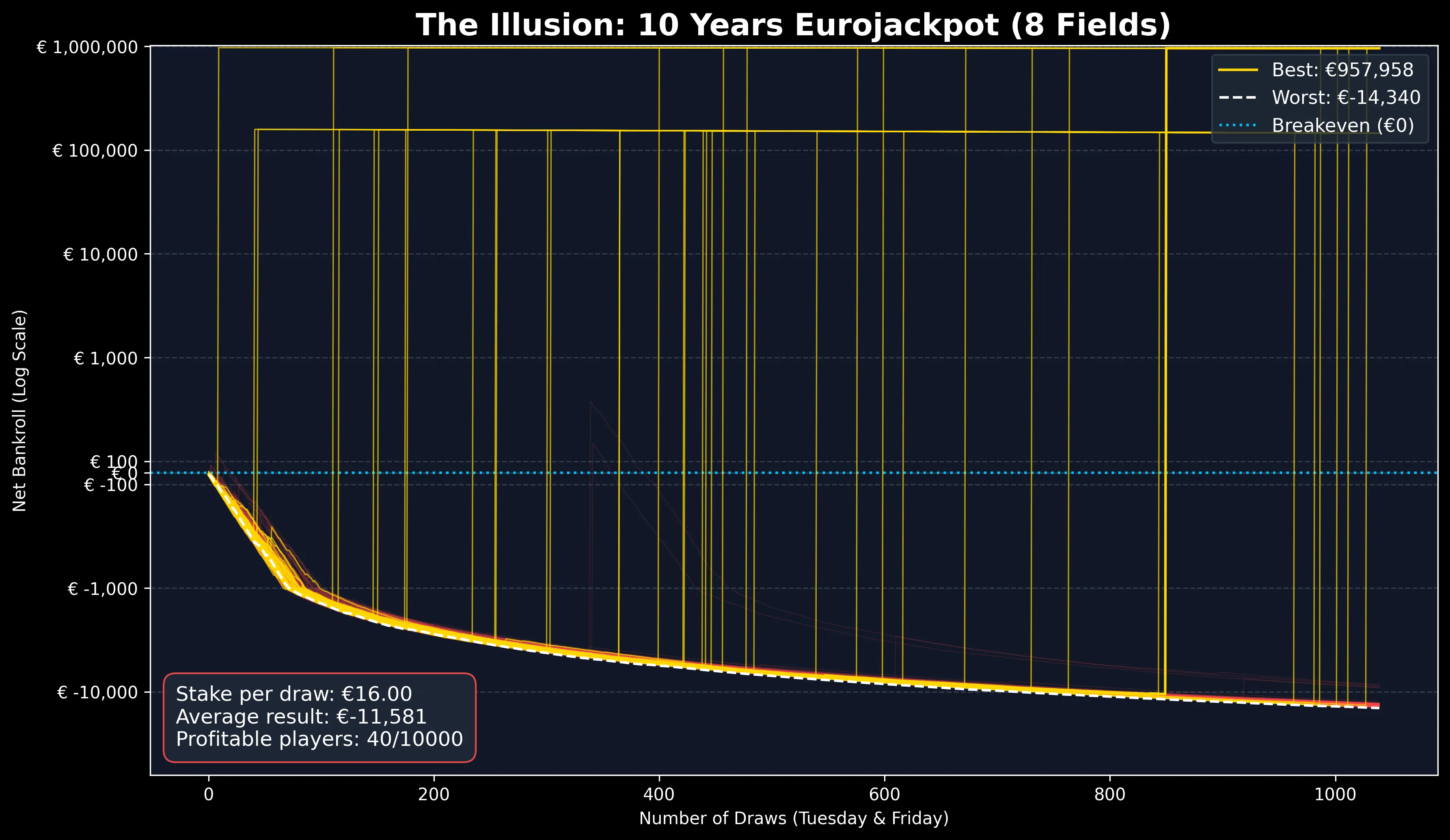
When you run the script, something visually striking happens. Thanks to the symlog scaling on the Y-axis, we get to see both: the brutal, steady losses of the general public and the absurd outliers of the extreme winners, all without breaking the chart.

The hard truth in numbers: At 8 lines per draw, you will burn through roughly €11,500 in 10 years. The simulation shows it clearly: even if you hit 3 correct numbers now and then, it won’t save you from the statistical expected value. The red cloud inevitably drags every player into the negative. Most of the time, not a single one of the 1,000 simulated players finishes the decade in the green.

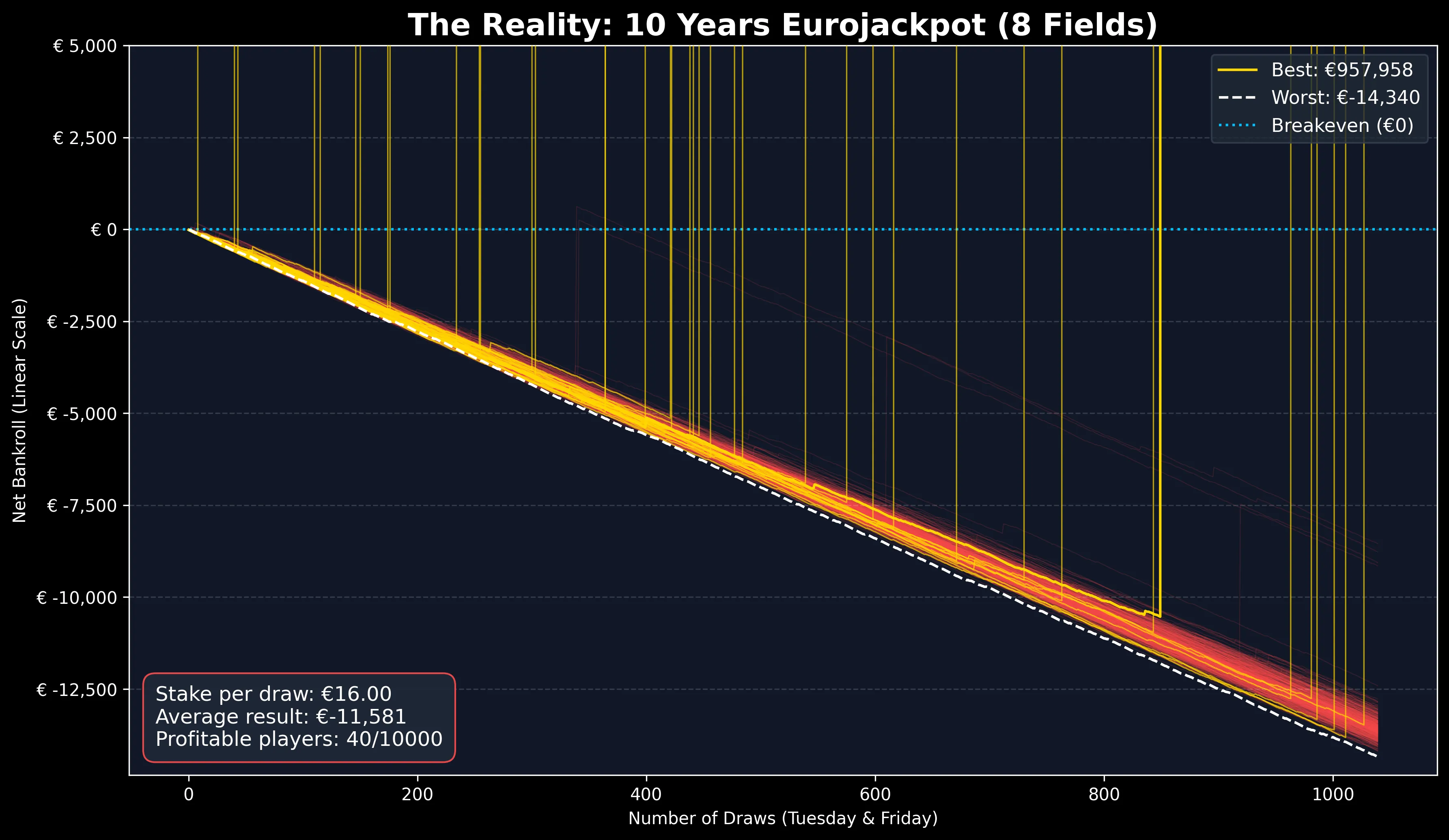
Think you’re that green outlier on the chart? Test your own 8 lucky lines in our Eurojackpot Simulator and click your way into bankruptcy!